Basic Usage Tutorial¶

Adam Klie (last updated: 07/08/2023)

In this tutorial, we illustrate a basic end-to-end EUGENe workflow that trains and interprets a single task regression model on a published dataset of plant promoters. If you are just starting out with EUGENE, you are in the right place! This tutorial will walk you through the steps of preparing the data, training a single task regression model, and interpreting that trained model.

You can also find this tutorial as a Jupyter notebook in the docs directory of the EUGENE repository. You can copy this notebook from there, or just copy and paste the code in each cell into a new notebook to follow along. Just make sure to have installed EUGENe in your environment before you start!

Warning: Before you start! Running this notebook without a GPU on this data is feasible but will be very slow. We’d recommend using Google Colab if you don’t have access to your own GPU.

Note: We’ve noticed that for some IDE configurations, plots do not render in a Jupyter notebook unless you include the %matplotlib inline magic command. If you are having trouble rendering plots, make sure you have this line in your notebook or use plt.show() after each plot.

[1]:

%matplotlib inline

Configuring¶

To make the sometimes painful process of keeping track of global parameters and input/output file paths easier, we usually like to set these through EUGENE’s settings up front. This will control the default directories for things like:

Data downloads with seqdatasets
Model configuration files (i.e. EUGENe will know where to look for these files without you having to specify the full path every time)
Model logs, checkpoints, and predictions
Figures and plots

These small quality of life features can go a long way to preserve your sanity!

[2]:

# Change this to where you would like to save all your results
import os
os.chdir("/cellar/users/aklie/projects/ML4GLand/tutorials/EUGENe")  # TODO: change this to your own directory
cwd = os.getcwd()
cwd

[2]:

'/cellar/users/aklie/projects/ML4GLand/tutorials/EUGENe'

[3]:

# Configure EUGENe directories, if you do not set these, EUGENe will use the default directories
from eugene import settings
settings.config_dir = "./tutorial_configs" # Directory to specify when you want to load a model from a config file
settings.dataset_dir = "./tutorial_dataset" # Directory where EUGENe will download datasets to
settings.logging_dir = "./tutorial_logs" # Directory where EUGENe will save Tensorboard training logs and model checkpoints to
settings.output_dir = "./tutorial_output" # Directory where EUGENe will save output files to
settings.figure_dir = "./tutorial_figures" # Directory to specify to EUGENe to save figures to

Dataloading¶

For this tutorial, we will reproduce the prediction of promoter activity featured in Jores et al., 2021 that uses DNA sequences as input to predict STARR-seq activity. We first need to load this dataset. If the dataset is a “EUGENe benchmarking dataset”, it can be loaded in through the SeqDatasets subpackage. Let’s load the package first

[4]:

import seqdatasets

OMP: Info #276: omp_set_nested routine deprecated, please use omp_set_max_active_levels instead.

We can next use the get_dataset_info() function to get information about the datasets available as “EUGENe benchmarking datasets”.

[5]:

# Check the dataset
seqdatasets.get_dataset_info()

[5]:

	n_seqs	n_targets	metadata	url	description	author
dataset_name
random1000	1000	1	10 randomly generated binary labels (label_{0-...	https://github.com/cartercompbio/EUGENe/tree/m...	A randomly generated set of 1000 sequences wit...	Adam Klie (aklie@eng.ucsd.edu)
ray13	241357	244	probe set (Probe_Set), bidning intensity value...	http://hugheslab.ccbr.utoronto.ca/supplementar...	This dataset represents an in vitro RNA bindin...	Hayden Stites (haydencooperstites@gmail.com)
farley15	163708	2	barcode (Barcode), RPMs from each biological r...	https://zenodo.org/record/6863861#.YuG15uxKg-Q	This dataset represents SEL-seq data of C. int...	Adam Klie (aklie@eng.ucsd.edu)
deBoer20	100000000+	1	Variable depending on chosen file	https://www.ncbi.nlm.nih.gov/geo/query/acc.cgi...	Gigantic parallel reporter assay data from ~10...	Adam Klie (aklie@eng.ucsd.edu)
jores21	147966	1	set (set), species (sp), gene promoter came fr...	https://raw.githubusercontent.com/tobjores/Syn...	This datast includes activity scores for 79,83...	Adam Klie (aklie@eng.ucsd.edu)
deAlmeida22	484052	4	Normalized enrichment scores for developmental...	https://zenodo.org/record/5502060/	This dataset includes UMI-STARR-seq data from ...	Adam Klie (aklie@eng.ucsd.edu)

We are in luck! The plant promoter dataset is available via the jores21() command. If you are requesting this dataset for the for the first time, it will be downloaded and loaded into a SeqData object automagically (and downloaded to your settings.dataset_dir).

[6]:

# Download the dataset to the dataset dir. We are using the promoters assayed in leaf promoters here
sdata = seqdatasets.jores21(dataset="leaf")
sdata

Dataset jores21 CNN_test_leaf.tsv has already been downloaded.
Dataset jores21 CNN_train_leaf.tsv has already been downloaded.
Zarr file found. Opening zarr file.

[6]:

<xarray.Dataset>
Dimensions:     (_sequence: 72158, _length: 170)
Dimensions without coordinates: _sequence, _length
Data variables:
    enrichment  (_sequence) float64 dask.array<chunksize=(1000,), meta=np.ndarray>
    gene        (_sequence) object dask.array<chunksize=(1000,), meta=np.ndarray>
    seq         (_sequence, _length) |S1 dask.array<chunksize=(1000, 170), meta=np.ndarray>
    set         (_sequence) object dask.array<chunksize=(1000,), meta=np.ndarray>
    sp          (_sequence) object dask.array<chunksize=(1000,), meta=np.ndarray>

If you want to learn more about how you can use EUGENe to read from your standard genomics file formats or how we represents datasets in memory and on disk, check out the SeqData section of the usage principles and the SeqData subpackage.

Data Visualization¶

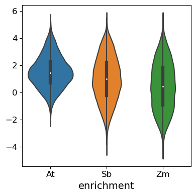
Data visualization is a key part of the EUGENe workflow. We can use the plot module to visualize aspects of our data such as the distribution of targets.

[7]:

from eugene import plot as pl

[8]:

# Plot the distribution of targets across the different species the promoters were derived from
pl.violinplot(sdata, vars=["enrichment"], groupby="sp", figsize=(4, 4))

Preprocessing¶

Now that we have our data loaded in, we can preprocess it using EUGENe’s preprocess module. This module wraps functionality from the SeqPro subpackage and includes several functions for common sequence preprocessing tasks.

Sequence preprocessing¶

Our first preprocessing step will be to one-hot encode our sequences. One-hot encoding is a common way to represent sequences as a matrix of 0s and 1s for model training. We will pass in DNA as the vocab explicitly, but this is the default if not specified.

[9]:

from eugene import preprocess as pp

[10]:

# One hot encode all the sequences in the sdata using the wrapper function
pp.ohe_seqs_sdata(sdata, alphabet="DNA")

Let’s also quickly set-up some identifiers for our sequences. This will come in handy during interpretation when we often want to visualize the importance of specific sequences.

[11]:

# Make unique ids for each sequence in the sdata
pp.make_unique_ids_sdata(sdata)

Dataset preprocessing¶

As is standard machine learning practice, we also need to split our data into training, validation, and test sets. This dataset comes with ‘train’ and ‘test’ labels in the ‘set’ annotation.

[12]:

# Split into train and test sets
sdata_train = sdata.sel(_sequence=(sdata["set"] == "train").compute())
sdata_test = sdata.sel(_sequence=(sdata["set"] == "test").compute())

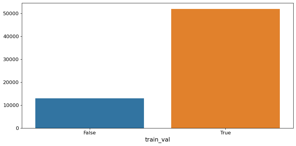
We also need to split the training sequences into train and validation sets. We can do this using EUGENe’s train_test_random_split function

[13]:

# Split the training set into training and validation
pp.train_test_random_split(sdata_train, dim="_sequence", train_var="train_val", test_size=0.2)

[14]:

# Check the split with a count plot
pl.countplot(sdata_train, vars="train_val", orient="h")

Training¶

Now that we have our data ready, it’s time to train our model! Training in EUGENe is done through the PyTorch Lightning (PL) framework. However PyTorch Lightning does not offer us much help with instantiating model architectures and initializing them. We will utilize EUGENE’s library of neural network parts and architectures to do this.

Instantiation and initialization¶

We first need to instantiate and initialize our model. We can use the models module to do this.

[15]:

from eugene import models

EUGENe offers several options for instantiating a model architecture. Here we will load in a Hybrid architecture that contains convoultional blocks that feed into recurrent layers, finishing with fully connected ones. We have set up a configuration file that trains pretty well on this dataset that you can download from here.

[16]:

# TODO: Uncomment and run the following to get the hybrid config downloaded
#!mkdir -p $cwd/tutorial_configs
#!wget https://raw.githubusercontent.com/adamklie/EUGENe_paper/revision/configs/jores21/hybrid.yaml -O $cwd/tutorial_configs/hybrid.yaml

We can then use the load_config function to load in this configuration file and initialize our model.

[17]:

model = models.load_config("hybrid.yaml")

We can also print out a summary of the model architecture using the summary function. Note that the configuration file we read in here also defines the LightningModule from PL that will be used to train the model. For more details on how this works, check out the tutorial on instantiating and initializing models.

[18]:

# Print out a summary of the model
model.summary()

Model: Hybrid
Sequence length: 170
Output dimension: 1
Task: regression
Loss function: mse_loss
Optimizer: Adam
        Optimizer parameters: {}
        Optimizer starting learning rate: 0.001
Scheduler: ReduceLROnPlateau
        Scheduler parameters: {'patience': 2}
Metric: r2score
        Metric parameters: {}
Seed: None
Parameters summary:

[18]:

  | Name         | Type    | Params
-----------------------------------------
0 | arch         | Hybrid  | 1.9 M
1 | train_metric | R2Score | 0
2 | val_metric   | R2Score | 0
3 | test_metric  | R2Score | 0
-----------------------------------------
1.9 M     Trainable params
0         Non-trainable params
1.9 M     Total params
7.703     Total estimated model params size (MB)

[19]:

# Initialize the weights
models.init_weights(model)

Model fitting¶

With a model intantiated and initialized, we are set up to fit our model to our plant promoters! We can do this through the train module in EUGENe

[20]:

from eugene import train

If you are using GPU accelerators on your machine, you can can use the gpus argument to set the number gpus you want to use. If left empty, EUGENe will try to infer the number of GPUs available. Training the model with a single GPU will take less than 5 minutes. Check out the API and docstring for the function below for more details on the arguments you can pass in.

[21]:

train.fit_sequence_module(
    model=model,
    sdata=sdata_train,
    seq_var="ohe_seq",
    target_vars=["enrichment"],
    in_memory=True,
    train_var="train_val",
    epochs=25,
    batch_size=128,
    num_workers=4,
    prefetch_factor=2,
    drop_last=False,
    name="hybrid",
    version="tutorial_model",
    transforms={"ohe_seq": lambda x: x.swapaxes(1, 2)}
)

Dropping 0 sequences with NaN targets.
Loading ohe_seq and ['enrichment'] into memory
No seed set

/cellar/users/aklie/opt/miniconda3/envs/ml4gland/lib/python3.9/site-packages/lightning_fabric/plugins/environments/slurm.py:165: PossibleUserWarning: The `srun` command is available on your system but is not used. HINT: If your intention is to run Lightning on SLURM, prepend your python command with `srun` like so: srun python /cellar/users/aklie/opt/miniconda3/envs/ml4gland/lib ...
  rank_zero_warn(
GPU available: True (cuda), used: True
TPU available: False, using: 0 TPU cores
IPU available: False, using: 0 IPUs
HPU available: False, using: 0 HPUs
/cellar/users/aklie/opt/miniconda3/envs/ml4gland/lib/python3.9/site-packages/lightning_fabric/plugins/environments/slurm.py:165: PossibleUserWarning: The `srun` command is available on your system but is not used. HINT: If your intention is to run Lightning on SLURM, prepend your python command with `srun` like so: srun python /cellar/users/aklie/opt/miniconda3/envs/ml4gland/lib ...
  rank_zero_warn(
LOCAL_RANK: 0 - CUDA_VISIBLE_DEVICES: [0]

  | Name         | Type    | Params
-----------------------------------------
0 | arch         | Hybrid  | 1.9 M
1 | train_metric | R2Score | 0
2 | val_metric   | R2Score | 0
3 | test_metric  | R2Score | 0
-----------------------------------------
1.9 M     Trainable params
0         Non-trainable params
1.9 M     Total params
7.703     Total estimated model params size (MB)

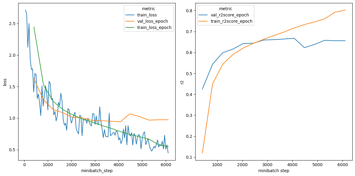
We can see how our models trained over time by plotting a training summary. All you need to do is point the training_summary function to your the EUGENe logging directory.

[36]:

# Plot a loss curve and an r2 curve as a metric
pl.training_summary(os.path.join(settings.logging_dir, "hybrid", "tutorial_model"), metric="r2")

Evaluation¶

After the model’s been trained, we can evaluate our performance on our held-out test data. This is done through the evaluate module.

[22]:

from eugene import evaluate

We want to use our best model for evaluation. We can see from the training curve above that our model began overfitting the data after about 3000 training steps. Lucky for us, PyTorch Lightning keeps track of our best model for us! We can load this model in from the log directory like so

[24]:

# We will use the glob Python library to help us find the path to our model
import glob

[25]:

# We point to the checkpoints directory within the logging directory to grab the best model
model_file = glob.glob(os.path.join(settings.logging_dir, "hybrid", "tutorial_model", "checkpoints", "*"))[0]
best_model = models.SequenceModule.load_from_checkpoint(model_file, arch=model.arch)

Our model is loaded in. Now let’s make some predictions

[26]:

# Use this best model to predict on the held-out data. This will store predictions in
evaluate.predictions_sequence_module(
    best_model,
    sdata=sdata_test,
    seq_var="ohe_seq",
    target_vars="enrichment",
    batch_size=2048,
    in_memory=True,
    name="hybrid",
    version="tutorial_model",
    file_label="test",
    prefix=f"tutorial_model_",
    transforms={"ohe_seq": lambda x: x.swapaxes(1, 2)}
)

Loading ohe_seq and ['enrichment'] into memory

/cellar/users/aklie/opt/miniconda3/envs/ml4gland/lib/python3.9/site-packages/lightning_fabric/plugins/environments/slurm.py:165: PossibleUserWarning: The `srun` command is available on your system but is not used. HINT: If your intention is to run Lightning on SLURM, prepend your python command with `srun` like so: srun python /cellar/users/aklie/opt/miniconda3/envs/ml4gland/lib ...
  rank_zero_warn(
GPU available: True (cuda), used: True
TPU available: False, using: 0 TPU cores
IPU available: False, using: 0 IPUs
HPU available: False, using: 0 HPUs
LOCAL_RANK: 0 - CUDA_VISIBLE_DEVICES: [0]
/cellar/users/aklie/opt/miniconda3/envs/ml4gland/lib/python3.9/site-packages/pytorch_lightning/trainer/connectors/data_connector.py:430: PossibleUserWarning: The dataloader, predict_dataloader, does not have many workers which may be a bottleneck. Consider increasing the value of the `num_workers` argument` (try 16 which is the number of cpus on this machine) in the `DataLoader` init to improve performance.
  rank_zero_warn(

By default, these predictions are automatically stored in the SeqData object:

We know have predictions from our trained model! Let’s look at a scatterplot to see how we did

[29]:

pl.performance_scatter(
    sdata_test,
    target_vars="enrichment",
    prediction_vars="tutorial_model_enrichment_predictions",
    alpha=0.5,
    groupby="sp",
    figsize=(8, 8)
)

Dropping 0 sequences with NaN targets.
Group R2 MSE Pearsonr Spearmanr
At 0.4709936799710689 0.736818682004814 0.6968483944361217
Sb 0.6154806217522697 1.04397699584586 0.8190967734520656
Zm 0.7056497647003188 0.8962513202149551 0.8426121671527911

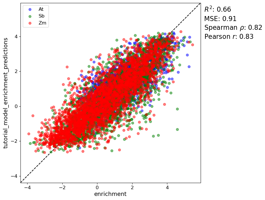
Not too shabby. We were able to train a pretty predictive model on this dataset with just DNA sequences as input!

Interpretation¶

Seeing good model performance is a big step in the right direction, but is far from the whole picture. We also want to try to better understand what our model is learning. We can do this through model interpretation. Model interpretation in EUGENe is done through the interpret module which relies heavily on functionality built into the SeqExplainer subpackage.

[30]:

from eugene import interpret

Filter interpretation¶

We will first get an idea of what each filter of first convoulional layer of the model is seeing by using the interpret module’s `generate_pfms_sdata <https://eugene-tools.readthedocs.io/en/latest/api/eugene.interpret.generate_pfms_sdata.html?highlight=generate_pfms#eugene.interpret.generate_pfms_sdata>`__ function. This creates a position frequency matrix for each filter in the model using sequences that highly activate that filter (can be defined in multiple ways). We often times pass the the test sequences through the model, but you can theoretically pass any sequences you want.

[33]:

interpret.generate_pfms_sdata(
    best_model,
    sdata_test,
    seq_var="ohe_seq",
    layer_name="arch.conv1d_tower.layers.1",
    kernel_size=13,
    num_filters=256,
    num_seqlets=100,
    transforms={"ohe_seq": lambda x: x.swapaxes(1, 2)}
)

Now let’s visualize a few of these PFMs to see if we can decipher what the filters are picking up on

[35]:

# We can visualize these PFMs as PWM logos
pl.multifilter_viz(
    sdata_test,
    filter_nums=range(0, 32),
    pfms_var="arch.conv1d_tower.layers.1_pfms",
    num_rows=8,
    num_cols=4,
    titles=[f"filter {i}" for i in range(0, 32)],
)

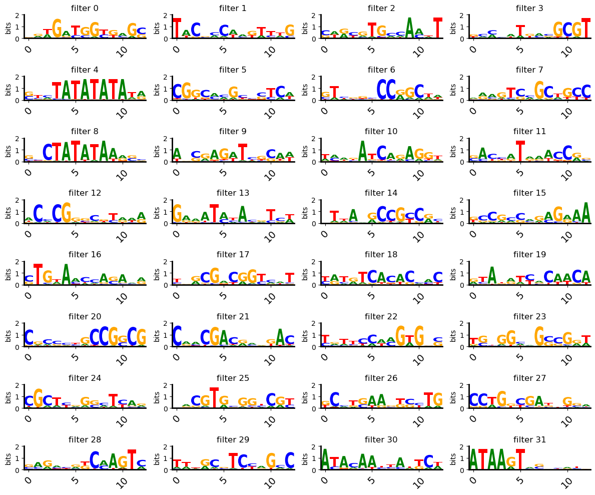
The qualitative visualization is nice, but often times we want to put some numbers behind what we are seeing. This is often done by annotating them PFMs from these filters against a database of known motifs with tools like TomTom. We offer a function for saving filters in an SeqData object to the MEME file format that can uploaded to the TomTom webtool.

[37]:

interpret.filters_to_meme_sdata(
    sdata_test,
    filters_var="arch.conv1d_tower.layers.1_pfms",
    axis_order=("_arch.conv1d_tower.layers.1_256_filters", "_ohe", "_arch.conv1d_tower.layers.1_13_kernel_size"),
    output_dir=os.path.join(settings.output_dir),
    filename="tutorial_model_best_model_filters.meme"
)

Output directory already exists: /cellar/users/aklie/projects/ML4GLand/tutorials/EUGENe/tutorial_output
Saved pfm in MEME format as: /cellar/users/aklie/projects/ML4GLand/tutorials/EUGENe/tutorial_output/tutorial_model_best_model_filters.meme

Note: Filters are not always interpretable to a human eye, or for that matter, to TomTom and databases of known motifs. The methods in this analysis are far from perfect, but can be a useful starting point for understanding what your model is learning. For more details on filter interpretation, check out the `filter interpretation tutorial <>`__.

Attribution analysis¶

We will next perform an analysis in which we quantify the contribution of each nucleotide of an input sequence to the model’s predictions for that sequence. This is called attribution analysis and can be performed in EUGENe with the attribute_sdata function. Here we will aply the DeepLIFT method to our best model on our held-out test sequences.

[38]:

interpret.attribute_sdata(
    best_model,
    sdata_test,
    method="DeepLift",
    batch_size=128,
    reference_type="zero",
    transforms={"ohe_seq": lambda x: x.swapaxes(1, 2)}
)

/cellar/users/aklie/opt/miniconda3/envs/ml4gland/lib/python3.9/site-packages/captum/attr/_core/deep_lift.py:336: UserWarning: Setting forward, backward hooks and attributes on non-linear
               activations. The hooks and attributes will be removed
            after the attribution is finished
  warnings.warn(
/cellar/users/aklie/opt/miniconda3/envs/ml4gland/lib/python3.9/site-packages/captum/attr/_core/deep_lift.py:467: UserWarning: An invalid module MaxPool1d(kernel_size=2, stride=2, padding=0, dilation=1, ceil_mode=False) is detected. Saved gradients will
                be used as the gradients of the module's input tensor.
                See MaxPool1d as an example.
  warnings.warn(

We can then visualize these importance scores using a sequence logo plot. Here we show the results on the sequences with the highest predicted activity by our model.

[39]:

# Grab the top3 in terms of predictions to plot tracks for
top3 = sdata_test["tutorial_model_enrichment_predictions"].to_series().sort_values(ascending=False).iloc[:3].index
ids = sdata_test["id"].values[top3]
pl.multiseq_track(
    sdata_test,
    seq_ids=ids,
    attrs_vars = "DeepLift_attrs",
    ylabs="DeepLift",
    height=3,
    width=40,
)

Note: There are many nuances to attribution analysis that we won’t get into here. For more details on how this works, check out the tutorial on attribution analysis.

Global importance analysis (GIA)¶

Another class of interpretation methods that are gaining a lot of traction in the field are those that involve designing experiments for the model in silico. The general idea is see what model predicts when we feed it sequences we design ourselves and compare that to some baseline set of predictions. There are no shortage of potential ideas of what sequence to feed the model, but test the positional importance of a TATA box motif.

We first need some background sequences to establish baseline predictions. Here we use the SeqPro subpackage to generate 5 random sequences and make our own SeqData object from scratch

[48]:

# Import the packages
import seqpro as sp
import xarray as xr

[51]:

# Create an SeqData object so its compatible with the function
random_ohe_seq = sp.ohe(sp.random_seqs((5, 170), sp.alphabets.DNA), sp.alphabets.DNA).swapaxes(1, 2)
sdata_random = xr.Dataset({"ohe_seq": (("_sequence", "_ohe", "length"), random_ohe_seq)})
pp.make_unique_ids_sdata(sdata_random, id_var="name")

[70]:

# Let's get our background predictions
sdata_random["background_predictions"] = best_model.predict(sdata_random["ohe_seq"].values).squeeze()

To handle the motif, we will use the MotifData subpackage in EUGENe.

[71]:

import motifdata as md

[72]:

# TODO: The motif can be downlaoded from https://github.com/tobjores/Synthetic-Promoter-Designs-Enabled-by-a-Comprehensive-Analysis-of-Plant-Core-Promoters/blob/main/data/misc
# !wget https://raw.githubusercontent.com/tobjores/Synthetic-Promoter-Designs-Enabled-by-a-Comprehensive-Analysis-of-Plant-Core-Promoters/main/data/misc/CPEs.meme -O $cwd/tutorial_dataset/CPEs.meme

[73]:

# We can load it and pull out the PFM and other info about the motif
meme = md.read_meme(os.path.join(settings.dataset_dir, "CPEs.meme"))
motif = meme.motifs["TATA"]
feat_name = motif.name
pfm = motif.pfm
consensus = motif.consensus
consensus_ohe = sp.ohe(consensus, alphabet=sp.alphabets.DNA)
feat_name, pfm, consensus

[73]:

('TATA',
 array([[0.1275, 0.3765, 0.1195, 0.3765],
        [0.1575, 0.3985, 0.199 , 0.2455],
        [0.249 , 0.303 , 0.197 , 0.251 ],
        [0.1235, 0.655 , 0.0755, 0.1455],
        [0.01  , 0.002 , 0.002 , 0.986 ],
        [0.968 , 0.    , 0.    , 0.032 ],
        [0.002 , 0.014 , 0.006 , 0.978 ],
        [0.992 , 0.    , 0.002 , 0.006 ],
        [0.653 , 0.012 , 0.002 , 0.333 ],
        [0.974 , 0.    , 0.008 , 0.018 ],
        [0.341 , 0.028 , 0.036 , 0.5955],
        [0.6955, 0.0815, 0.1195, 0.1035],
        [0.1255, 0.432 , 0.3165, 0.1255],
        [0.291 , 0.418 , 0.175 , 0.1155],
        [0.263 , 0.3445, 0.1755, 0.2175],
        [0.307 , 0.3085, 0.2365, 0.1475]]),
 'CCCCTATAAATACCCC')

Now that we have a feature, we can implant it at every possible position of the input sequence and see what that does to model predictions.

[74]:

# This is the EUGENe function that does exactly that!
interpret.positional_gia_sdata(
    model=best_model,
    sdata=sdata_random,
    feature=consensus_ohe,
    id_var="name",
    store_var=f"slide_{feat_name}",
    encoding="onehot"
)

Next we can visualize the results as a line plot using a custom function from the plot module.

[75]:

ax = pl.positional_gia_plot(sdata_random, vars=[f"slide_{feat_name}"], id_var="name", return_axes=True)
ax.hlines(sdata_random["background_predictions"].mean(), 0, 170, linestyle="--", color="red")

[75]:

<matplotlib.collections.LineCollection at 0x1552f4de7280>

Sequence generation¶

The last class of interpretability methods currently offered in EUGENe uses trained models to guide sequence evolution. We implement the simplest form of this approach that iteratively evolves a sequence by greedily inserting the mutation with the largest predicted impact at each iteration. Starting with an initial sequence (e.g. random, shuffled, etc.), this strategy can be used to evolve synthetic functional sequences.. This style of analysis is a promising direction for further research, and can also serve as an extension of ISM for validating that the model has learned representations that resemble motifs.

[76]:

# Evolve this sequence for ten rounds
interpret.evolve_seqs_sdata(model=best_model, sdata=sdata_random, rounds=10)

[77]:

# Get all the vars that start with "evolved"
evolved_vars = ["original_score"] + [var for var in sdata_random.data_vars if var.startswith("evolved") and var.endswith("score")]

[78]:

# Check the predicted value at each round of evolution
sdata_random[evolved_vars].to_dataframe()

[78]:

	original_score	evolved_1_score	evolved_2_score	evolved_3_score	evolved_4_score	evolved_5_score	evolved_6_score	evolved_7_score	evolved_8_score	evolved_9_score	evolved_10_score
_sequence
0	-1.315275	2.592115	3.100401	3.349671	3.460264	3.541673	3.616242	3.676543	3.730854	3.782861	3.828243
1	0.189355	2.067887	2.389756	2.620612	2.820599	3.023727	3.195810	3.356424	3.472401	3.561384	3.628919
2	-0.042155	2.275804	2.780840	3.111794	3.352813	3.516827	3.620399	3.701992	3.768886	3.820019	3.869473
3	1.054857	2.884281	3.528840	3.969130	4.079750	4.169396	4.253009	4.303516	4.341343	4.378622	4.411158
4	0.727182	1.760178	2.622345	2.959457	3.077595	3.174875	3.257919	3.318932	3.371122	3.416539	3.460763

Wrapping up¶

That concludes our basic usage tutorial! We hope you found it helpful. Don’t hesitate to raise a GitHub issue if you run into any errors or if anything is overly confusing!

You can find tutorials dedicated to many of the specific steps shown here on the tutorials repo (https://github.com/ML4GLand/tutorials)